Create a radar plot for MX metrics relating to each day of the measurement of physical behavior

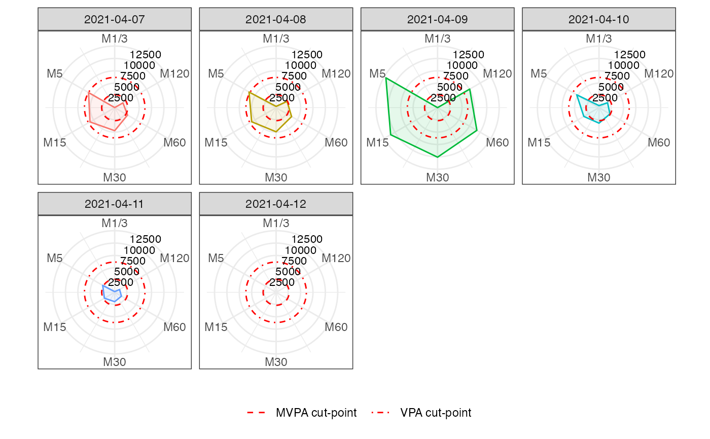
This function creates radar plots in relation to MX metrics as illustrated in Rowlands et al. (2018; doi:10.1249/MSS.0000000000001561) paper, here for each day of an accelerometer measurement.

Usage

create_fig_mx_by_day(
  data,
  labels = NULL,
  mpa_cutpoint = 2690,
  vpa_cutpoint = 6167
)

Arguments

data: A dataframe with physical behavior metrics summarised for each day of the measurement. It should have been obtained using the prepare_dataset, mark_wear_time, mark_intensity, and then the recap_by_day functions.
labels: A vector of numeric values setting the breaks of the Y axis of the radar plot. Default is a vector of 6 values with a start at 0 and an end at the maximum of all the computed MX metrics.
mpa_cutpoint: A numeric value at and above which time is considered as spent in moderate-to-vigorous physical activity (in counts/epoch length used to compute MX metrics). Default value is from Sasaki et al. (2011; doi:10.1016/j.jsams.2011.04.003) relating to vector magnitude in counts/min.
vpa_cutpoint: A numeric value at and above which time is considered as spent in vigorous physical activity (in counts/epoch length used to compute MX metrics). Default value is from Sasaki et al. (2011; doi:10.1016/j.jsams.2011.04.003) relating to vector magnitude in counts/min.

Value

A ggplot object

Examples

# \donttest{
file <- system.file("extdata", "acc.agd", package = "activAnalyzer")
mydata <- prepare_dataset(data = file)
mydata_with_wear_marks <- mark_wear_time(
    dataset = mydata, 
    TS = "TimeStamp", 
    to_epoch = 60,
    cts  = "vm",
    frame = 90, 
    allowanceFrame = 2, 
    streamFrame = 30
    )
#> frame is 90
#> streamFrame is 30
#> allowanceFrame is 2
mydata_with_intensity_marks <- mark_intensity(
    data = mydata_with_wear_marks, 
    col_axis = "vm", 
    equation = "Sasaki et al. (2011) [Adults]",
    sed_cutpoint = 200, 
    mpa_cutpoint = 2690, 
    vpa_cutpoint = 6167, 
    age = 32,
    weight = 67,
    sex = "male"
    )
#> You have computed intensity metrics with the mark_intensity() function using the following inputs: 
#>     axis = vm
#>     sed_cutpoint = 200 counts/min
#>     mpa_cutpoint = 2690 counts/min
#>     vpa_cutpoint = 6167 counts/min
#>     equation = Sasaki et al. (2011) [Adults]
#>     age = 32
#>     weight = 67
#>     sex = male
summary_by_day <- recap_by_day(
    data = mydata_with_intensity_marks, 
    col_axis = "vm",
    age = 32, 
    weight = 67, 
    sex = "male",
    valid_wear_time_start = "07:00:00",
    valid_wear_time_end = "22:00:00",
    start_first_bin = 0,
    start_last_bin = 10000,
    bin_width = 500
    )$df_all_metrics
#> Joining with `by = join_by(date)`
#> Joining with `by = join_by(date)`
#> Joining with `by = join_by(date)`
#> You have computed results with the recap_by_day() function using the following inputs: 
#>          age = 32
#>          weight = 67
#>          sex = male
create_fig_mx_by_day(
    data = summary_by_day,
    labels = seq(2500, 12500, 2500)
)

# }