Compute intensity distribution metrics — compute_intensity_distri

This function computes metrics that describe the distribution of intensity for each day of a dataset. Computations are performed based on the daily periods set for analysis and on the detected wear time.

Usage

compute_intensity_distri_metrics(
  data,
  col_axis = "vm",
  col_time = "time",
  valid_wear_time_start = "00:00:00",
  valid_wear_time_end = "23:59:59",
  start_first_bin = 0,
  start_last_bin = 10000,
  bin_width = 500
)

Arguments

data: A dataframe obtained using the prepare_dataset, mark_wear_time, and then the mark_intensity functions.
col_axis: A character value to indicate the name of the variable to be used to compute total time per bin of intensity.
col_time: A character value to indicate the name of the variable to be used to determine the epoch length of the dataset.
valid_wear_time_start: A character value with the HH:MM:SS format to set the start of the daily period that will be considered for computing metrics.
valid_wear_time_end: A character value with the HH:MM:SS format to set the end of the daily period that will be considered for computing metrics.
start_first_bin: A numeric value to set the lower bound of the first bin of the intensity band (in counts/epoch duration).
start_last_bin: A numeric value to set the lower bound of the last bin of the intensity band (in counts/epoch duration).
bin_width: A numeric value to set the width of the bins of the intensity band (in counts/epoch duration).

Value

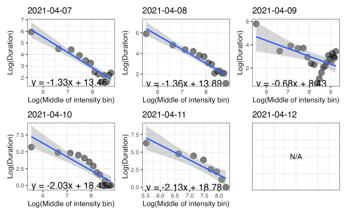
A list of objects: metrics, p_band, and p_log. metrics is a dataframe containing the intensity gradients and the MX metrics (in counts/epoch duration used) as described in Rowlands et al. (2018; doi:10.1249/MSS.0000000000001561). The graphic p_band shows the distribution of time spent in the configured bins of intensity for each day of the dataset. The graphic p_log shows, for each day, the relationship between the natural log of time spent in each bin with the natural log of the middle values of the intensity bins.

Examples

# \donttest{
file <- system.file("extdata", "acc.agd", package = "activAnalyzer")
mydata <- prepare_dataset(data = file)
mydata_with_wear_marks <- mark_wear_time(
    dataset = mydata, 
    TS = "TimeStamp", 
    to_epoch = 60,
    cts  = "vm",
    frame = 90, 
    allowanceFrame = 2, 
    streamFrame = 30
    )
#> frame is 90
#> streamFrame is 30
#> allowanceFrame is 2
mydata_with_intensity_marks <- mark_intensity(
    data = mydata_with_wear_marks, 
    col_axis = "vm", 
    equation = "Sasaki et al. (2011) [Adults]",
    sed_cutpoint = 200, 
    mpa_cutpoint = 2690, 
    vpa_cutpoint = 6167, 
    age = 32,
    weight = 67,
    sex = "male"
    )
#> You have computed intensity metrics with the mark_intensity() function using the following inputs: 
#>     axis = vm
#>     sed_cutpoint = 200 counts/min
#>     mpa_cutpoint = 2690 counts/min
#>     vpa_cutpoint = 6167 counts/min
#>     equation = Sasaki et al. (2011) [Adults]
#>     age = 32
#>     weight = 67
#>     sex = male
compute_intensity_distri_metrics(
   data = mydata_with_intensity_marks,
   col_axis = "vm",
   col_time = "time",
   valid_wear_time_start = "00:00:00",
   valid_wear_time_end = "23:59:59",
   start_first_bin = 0,
   start_last_bin = 10000,
   bin_width = 500
    )
#> Joining with `by = join_by(date)`
#> $metrics
#>         date    ig   M1/3    M120     M60      M30      M15       M5
#> 1 2021-04-07 -1.33  80.33 1998.67 3054.71  4721.17  5828.83  6160.10
#> 2 2021-04-08 -1.36 323.79 2619.29 3671.61  4944.65  5763.85  6385.89
#> 3 2021-04-09 -0.68  66.66 7560.33 9226.30 10066.52 10999.13 12113.34
#> 4 2021-04-10 -2.03 477.97 2063.99 2612.85  3196.95  3603.35  5263.99
#> 5 2021-04-11 -2.13 200.89 1202.82 1635.32  1963.83  2458.20  2870.01
#> 6 2021-04-12    NA     NA      NA      NA       NA       NA       NA
#> 
#> $p_band

#> 
#> $p_log
#> `geom_smooth()` using formula = 'y ~ x'
#> `geom_smooth()` using formula = 'y ~ x'
#> `geom_smooth()` using formula = 'y ~ x'
#> `geom_smooth()` using formula = 'y ~ x'
#> `geom_smooth()` using formula = 'y ~ x'

#> 
 # }